Metabarcoding to identify organisms from environmental DNA (eDNA)
Metabarcoding is a high-throughput sequencing approach used to identify the diversity of organisms in environmental samples. It uses a specific gene fragment: typically COX-I mitochondrial genes for eukaryotes, and the 16S rRNA gene for bacteria. Bioinformatics tools then help to analyze the data and identify the organisms present in the sample. One commonly used tool for this purpose is BLAST: it allows for comparison of sequences to reference databases and identifies the closest matches. In this tutorial, we will go through the steps of using BLAST with SequenceServer to identify organisms in environmental samples.
The variable regions of the 16S rRNA gene contain species-specific sequences that allow for the identification of different bacterial taxa, making it a commonly used method to characterize bacterial communities. We will analyze a 16S rRNA gene amplicon sequence dataset generated from a study aimed at characterizing the microbiome composition of infant gut (Khonsari et al., 2016). The OTUs were generated by sequencing a PCR-amplified fragment of the 16S rRNA using the following method:
- DNA extraction from infant feces sample.
- PCR-amplification of the 16S rRNA region with universal primers (this generates “amplicons”)
- Purification and quantification of PCR product that is approximately 450 nucleotides long.
- Illumina Library preparation.
- High-throughput sequencing Illumina paired-end platform, obtaining pairs of 250-bp long reads.
- Pre-processing of the obtained metagenomic amplicon data (quality and primer trimming, overlap merging, clustering by 97% similarity and filtering by length).
The final, clustered dataset comprises 271 sequences ranging between 440-460 bp in length. The names of the sequences also include their coverage (i.e., the number of reads clustered by similarity). These 271 sequences represent our operational taxonomic units (OTUs) of unknown identity. We will classify their taxonomy with BLAST.
Retrieving 16S rRNA database and starting up SequenceServer
Firstly, we need a 16S rRNA database of known species to perform BLAST searches on our OTUs. The NCBI provides publicly available sequences and curated databases, including the 16S rRNA. This database is also among the generic databases that SequenceServer Cloud BLAST users can simply select for their instance (other generic databases include 18S sequences, COX1 sequences, UnirRef50, and hg38). Alternatively, a FASTA format text file of 16S sequences, or a preformatted BLAST database can be added to any SequenceServer instance. SequenceServer automatically formats FASTA files into BLAST databases.
BLAST OTUs (Operational Taxonomic Units)
Opening SequenceServer in a web browser presents the following homepage, where the 16S database can be selected.
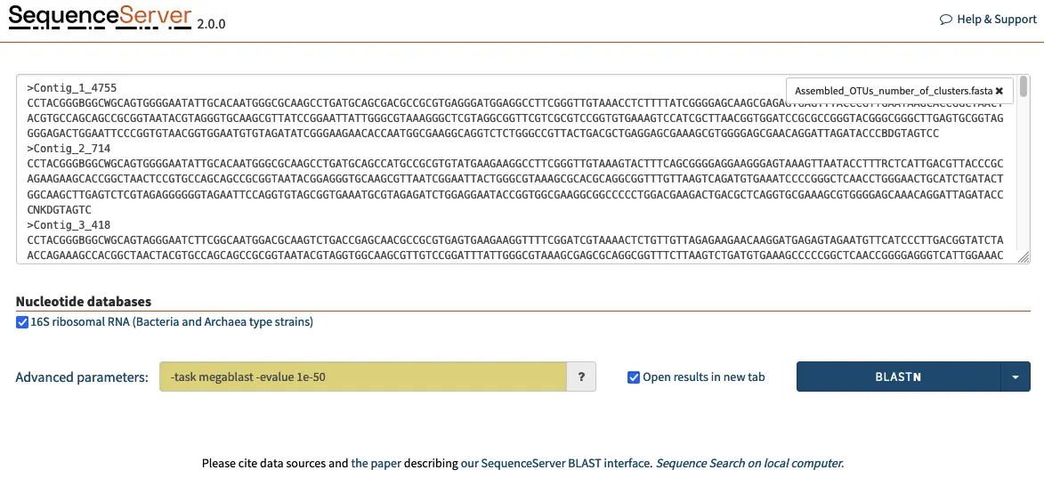
To begin identifying the 16S rRNA amplicon OTUs, we can input the queries in FASTA format in the dialog box and adjust parameters such as BLAST algorithm, E-value cut-off, scoring matrix and others. For our purposes where we are looking for high similarity we select the megablast algorithm and a E-value of 1e-50. This ensures that the query will run rapidly and only identify hit sequences that are highly similar to our queries.
Beware: A common strategy is to use the flag max_target_seq, with many authors setting this flag to 1 to limit BLAST output to only the best hit. However, this flag simply returns the first hit, which is not necessarily the best one as it depends on the order in which the sequences occur in the database. This leads to invalid analytic results Shah *et al.,* 2018. The –max_target_seq 1 approach should thus be avoided except in exceptional circumstances.
Our strategy differs in that we limit the output to only hits over an E-value threshold of 1e-50. We can then filter the “true” top hit with a simple R script. We are also using the megablast algorithm, which is more optimized for intraspecies comparison.
-task megablast -evalue 1e-50
The results of the BLAST search will be presented in a web page with information for each query, such as Contig_1, Contig_2, and so on, and their best hits.
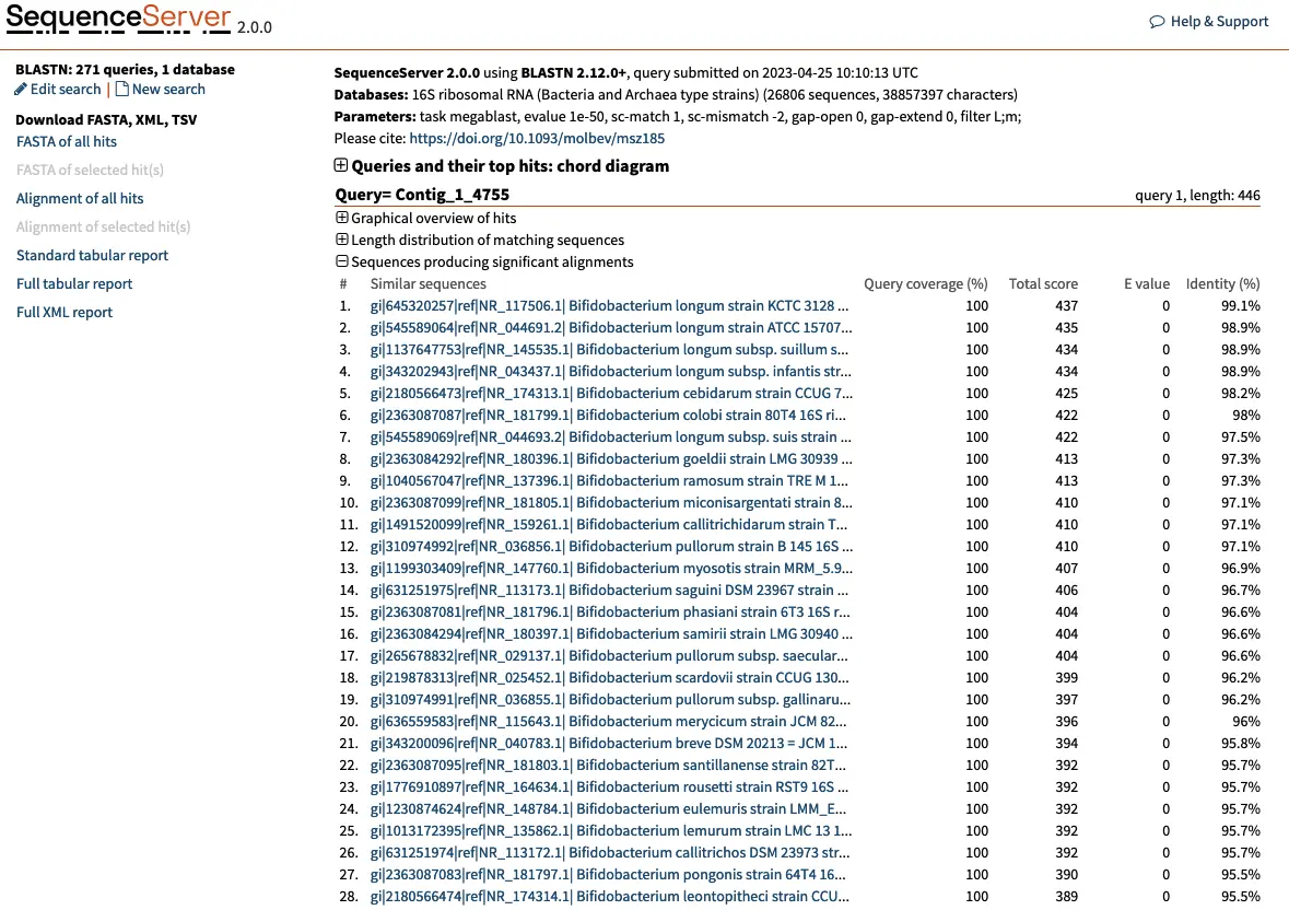
Let’s take Contig_1_4755 as an example. This contig represents the consensus of 4,755 reads clustered by 97% similarity. The best hit for this OTU is the 16S rRNA of Bifidobacterium longum strain KCTC 3128, with 100% query coverage, a total score of 435, a strong E-value (< 1e-100) and a 99.1% identity. We can be reasonably confident that this OTU is a Bifidobacterium longum. Selecting this first hit reveals more information:
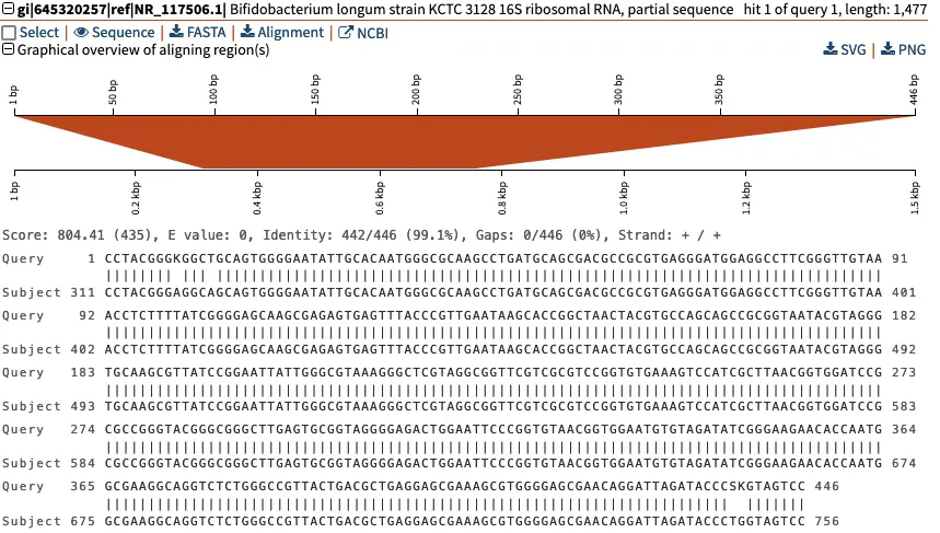
This detailed view shows the pairwise alignment between our “Query” sequence, Contig_1, and the “Subject” sequence fromBifidobacterium longumstrain KCTC that has the GenBank identifier
gi|645320257|ref|NR_117506.1. The middle line indicates|whenever the two sequences are identical. Here, we can see that that three of the nucleotide-level differences in sequence involve ambiguous nucleotides (“K” at position 9, and “S” and “K” around position 440). This ambiguity can arise for multiple reasons during the sequencing reaction.
Above the graphical overview of aligning region(s), clicking on the “NCBI” button will direct us to the NCBI page of the 16S rRNA reference sequence of Bifidobacterium longum. We can also download the sequence directly by clicking “FASTA”.
Retaining only the top hit for each query in R
The initial BLAST results yielded an overwhelming number of hits, with 500 hits per query for a total of 271 OTUs. Reviewing all of them manually would be time-consuming and unnecessary, as we are only interested in the top hit for each query. To do this, we can retrieve the full tabular report from SequenceServer (this is the equivalent of running BLAST with -outfmt 16 option). This table contains many columns, so we need to do some clean-up to make it more manageable. R works very well for this. We walk through the analysis step by step. If you want to try it yourself, feel free to grab the entire R script and the example dataset.
First, we need to load the libraries that we are going to use in R:
library(dplyr)
library(ggplot2)
library(stringr)
Next, we load the table in R and name the headers:
blast_results_file_tsv = "sequenceserver-full_tsv_report.tsv"
blast_results <- read.delim(blast_results_file_tsv, header = FALSE, comment.char = "#")

blast_results_header <- grep(pattern = "# Fields:", x = readLines(con = blast_results_file_tsv, n = 10), value = TRUE)[1]
blast_results_header <- sub(pattern = "# Fields: ", replacement = "", x = blast_results_header)
blast_results_colnames <- unlist(strsplit(x = blast_results_header, split = ", "))
blast_results_colnames <- gsub(pattern = " ", replacement = "_", x = blast_results_colnames)
colnames(blast_results) <- blast_results_colnames
The subject title column contains the name of the organism, but other information as well. We only want to keep the name and also replace spaces with underscores to prevent possible issues. We can enter this command in R to do just that:
blast_results$taxon <- gsub(x = blast_results$`subject_title`,
    pattern = "([A-z0-9]+ [A-z0-9]+).*",
    replacement = "\\1",
    perl = TRUE)
Next, we sort the BLAST output by query_id and bit_score in descending order, and select only the top hit for each group using the slice_head() function (this allows us to keep only the best hit for each query):
top_hits <- blast_results %>%
    arrange(query_id, desc(bit_score)) %>%
    group_by(query_id) %>%
    slice_head(n = 1) %>%
    arrange(desc(bit_score))
Classify taxonomy and plot results with ggplot2
Our BLAST output is now filtered and only reports the best hit for each OTUs/query.
We can then count the number of hits for each taxonomic group using the table() function and plot our results with ggplot2 :
taxa_count <- table(top_hits$taxon)
taxa_count_df <- data.frame(taxa = names(taxa_count), counts = as.numeric(taxa_count))
taxa_count_df <- taxa_count_df[order(-taxa_count_df$counts), ]
ggplot(taxa_count_df, aes(x = reorder(taxa, -counts), y = counts)) +
  geom_histogram(stat = "identity", fill = "#c74f14") +
  theme(axis.text.x = element_text(angle = 90, hjust = 1)) +
  xlab("Taxonomic group") +
  ylab("Number of hits")
Figure 1: Taxonomic classification of 271 OTUs and their number of hits
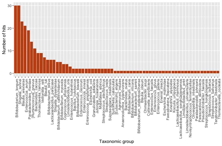
The results of our taxonomic classification indicate that Bifidobacterium longum is the dominant species in the sample. Bifidobacterium longum is one of the first types of bacteria to colonize the infant gut, and it plays an important role in shaping the development of the gut microbiome (Khonsari et al., 2016). Other Bifidobacterium species, in addition to Blautia, Enterococcus and Lacticaseibacillus are also commonly found in the gut microbiome of infants (Khonsari et al., 2016). Therefore, our results agree with the published literature.
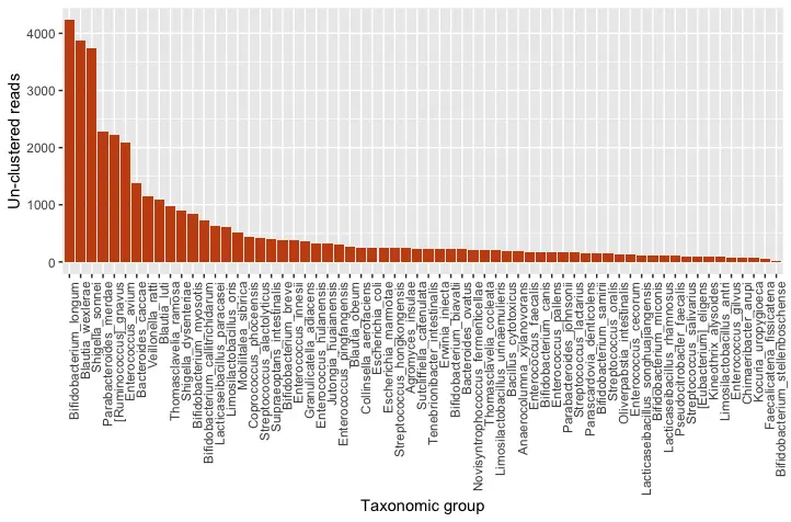
We can go one step further and incorporate the information on the number of reads clustered for each contig/OTUs in our histogram:
top_hits$clusters <- str_extract(top_hits$query_id, "\\d+$")

taxa_count_clusters <- top_hits %>%
  group_by(taxon) %>%
  summarise(clusters_sum = sum(as.numeric(clusters))) %>%
  arrange(desc(clusters_sum))

ggplot(taxa_count_clusters, aes(x = reorder(taxon, -clusters_sum), y = clusters_sum)) +
  geom_bar(stat = "identity", fill = "#c74f14") +
  theme(axis.text.x = element_text(angle = 90, hjust = 1)) +
  xlab("Taxonomic group") + ylab("Un-clustered reads")
Figure 2: Quantitative taxonomic classification of the full, un-clustered amplicon
Great job! You have successfully analyzed the gut microbiome data using SequenceServer and R. In this process, you have gained experience in several key areas, including data pre-processing, quality control, taxonomic classification, and visualization. By analyzing the data, you were able to identify the dominant bacterial species in the sample. In this case, the findings are consistent with published literature. Remember that bioinformatics is an ever-evolving field, and there is always more to learn. I encourage you to continue exploring and experimenting with different tools and techniques to deepen your understanding of the field. Good luck with your future endeavors!
References:
Khonsari, S., Suganthy, M., Burczynska, B., Dang, V., Choudhury, M. and Pachenari, A. (2016) ‘A comparative study of bifidobacteria in human babies and adults.’, Bioscience of microbiota, food and health. Japan, 35(2), pp. 97–103. doi: 10.12938/bmfh.2015-006.
Shah, N., Nute, M. G., Warnow, T. and Pop, M. (2019) ‘Misunderstood parameter of NCBI BLAST impacts the correctness of bioinformatics workflows’, Bioinformatics, 35(9), pp. 1613–1614. doi: 10.1093/bioinformatics/bty833.
R script
# Loading libraries
library(dplyr)
library(ggplot2)
library(stringr)

# Loading data
blast_results_file_tsv = "sequenceserver-full_tsv_report.tsv"
blast_results <- read.delim(blast_results_file_tsv, header = FALSE, comment.char = "#")

blast_results_header <- grep(pattern = "# Fields:", x = readLines(con = blast_results_file_tsv, n = 10), value = TRUE)[1]
blast_results_header <- sub(pattern = "# Fields: ", replacement = "", x = blast_results_header)
blast_results_colnames <- unlist(strsplit(x = blast_results_header, split = ", "))
blast_results_colnames <- gsub(pattern = " ", replacement = "_", x = blast_results_colnames)
colnames(blast_results) <- blast_results_colnames

# Pulling out species name from the long description
blast_results$taxon <- gsub(x = blast_results$`subject_title`,
  pattern = "([A-z0-9]+ [A-z0-9]+).*",
  replacement = "\\1",
  perl = TRUE)

# Sorting BLAST output and retaining only the top hit
top_hits <- blast_results %>%
  arrange(query_id, desc(bit_score)) %>%
  group_by(query_id) %>%
  slice_head(n = 1) %>%
  arrange(desc(bit_score))

# Counting the number of unique taxa and plotting results
taxa_count <- table(top_hits$taxon)
taxa_count_df <- data.frame(taxa = names(taxa_count), counts = as.numeric(taxa_count))
taxa_count_df <- taxa_count_df[order(-taxa_count_df$counts), ]
ggplot(taxa_count_df, aes(x = reorder(taxa, -counts), y = counts)) +
  geom_histogram(stat = "identity", fill = "#c74f14") +
  theme(axis.text.x = element_text(angle = 90, hjust = 1)) +
  xlab("Taxonomic group") +
  ylab("Number of hits")


# Quantitative taxonomic classification of the full un-clustered amplicon
top_hits$clusters <- str_extract(top_hits$query_id, "\\d+$")

taxa_count_clusters <- top_hits %>%
  group_by(taxon) %>%
  summarise(clusters_sum = sum(as.numeric(clusters))) %>%
  arrange(desc(clusters_sum))

ggplot(taxa_count_clusters, aes(x = reorder(taxon, -clusters_sum), y = clusters_sum)) +
  geom_bar(stat = "identity", fill = "#c74f14") +
  theme(axis.text.x = element_text(angle = 90, hjust = 1)) +
  xlab("Taxonomic group") + ylab("Un-clustered reads")
Stay up to date
To receive the latest news from our team, enter your email: